
Send this article to a friend:
December
13
2019

|
Send this article to a friend: December |
|
Statistical misdirection
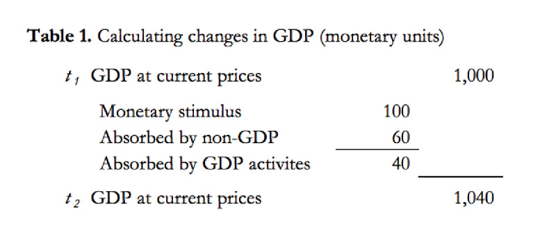
With the dollar tied to gold, there was no doubt about how the collapse in demand affected asset, commodity and consumer prices ninety years ago. If the turn of the current cycle leads to a similar outcome, it is unlikely to be properly reflected in official statistics for GDP. This article explains why GDP is a statistical fallacy, and the use of an inflation deflator is not only inappropriate but has been manipulated to produce an outcome that wrongly attributes success to monetary policies. Therefore, if an economic slump follows the coming credit crisis, it is unlikely to be reflected in these key government statistics. At some point, markets will stop believing in macroeconomics and adjust to the reality that governments are simply using monetary inflation as a means of funding increasing deficits. Then, interest rates will no longer be captives of the central banks but will rise to reflect the falling purchasing power of fiat currencies. Introduction There is little doubt that the global economy is entering a period of economic contraction. Surveys of business opinion around the world and declining trade volumes point to it as well as a basic comprehension of credit cycles. Anyone who doesn’t think Germany, a bell-whether manufacturer and exporter whose largest market is China, is slipping into economic contraction ignores simple evidence. And central bankers are all in easing mode, telling us that whatever they say in public, in private they see the same thing. On several occasions I have pointed out the alarming similarities between our current economic state and that of 1929, which led into the Wall Street crash. The commonality between then and now is the confluence of the peak of the credit cycle with increasing trade tariffs. But we should note there are two major differences: before the dollar’s devaluation in January 1934, prices of assets and goods expressed in dollars were all tied to gold at $20.67 to the ounce. And when demand for first assets, then goods contracted, the effect on their prices was clear: the Dow lost 89% from top to bottom, and producers’ prices roughly halved. Today, by fully exploiting the absence of gold backing central banks are on a mission to prevent prices falling by inflating the money quantity by however much it might take. This brings us to the second difference. The statistics which recorded the crash and the depression that followed were relatively straightforward. At the time, economists based their analyses on a few hard facts and relatively sound economic theories. But by the mid-1930s, US economist Simon Kuznets began formulating a statistical method for measuring the whole economy. His proposed measure, gross national product, then evolved into gross domestic product. The concept, as Kuznets himself argued, should only be used in context. But the growing influence of Keynes and other fellow travellers in the new field of macroeconomics meant it was not long before Kuznets’ cautions were ignored. Since then, statistics produced by government departments have expanded to provide dodgy evidence for Keynes’s new macroeconomics, which he had devised in order to escape the strictures of classical economics. The basis of government statistics was increasingly slanted towards purposes other than pure knowledge. For all the governments that went pure fiat and pure Keynesian in the 1970s, statistical corruption has evolved into a control mechanism to suppress the evidence of the economic condition of the day and the continual loss of purchasing power for currencies at rates higher than officially admitted. After prices were stabilised by massive interest rate increases in the late seventies and early eighties, government corruption of statistics increased apace. It was as if designed to reduce the cost of indexation, promised to users of government services and state pensioners alike. This apparently deliberate process has continued for nearly forty years and left us with economists and asset managers ignorant of the degree of statistical corruption, and beholden to the macroeconomic theories which inflates the values of their investments. This article attempts to knock some sense into this world of state-driven statistical corruption and groupthink in the investment industry by pointing out why two key statistics, GDP and CPI, are misleading. Given the increasing certainty of a worldwide economic slump and the growing prospects for an acceleration of monetary inflation to conceal the effects, maintaining personal wealth will require a comprehensive understanding how these statistics are being used to protect governments at the expense of their electors. GDP In order to fully understand the fallacy behind the use of gross domestic product to determine the state of the economy, one must appreciate the difference between progress and what has become to be described as economic growth. This difference was outlined by the Austrian economist, Ludwig von Mises, when he defined an evenly rotating economy. This is an imaginary construction, in which all transactions and physical conditions are repeated without change in each similar cycle of time. Everything is imagined continuing exactly as before, including all human ideas and goals. Under these fictitious constant and repetitive conditions there can be no net change in supply and demand and therefore there cannot be any change in prices.[i] It is worth examining the consequences of using this imaginary construction, because it forms the basis for the GDP model. It is an accounting device, which captures an economy at a moment in time, just as a company’s annual profit statement tell us its sales, expenses and profits. It allows the shareholders to take stock, as it were, and make comparisons. But the shareholders and management of any enterprise know that the following year will be different. There will be new markets to explore, while some existing markets wither, and customers are gained and lost. There will be new technologies, new competitors. Trade is a dynamic condition. An economy is equally dynamic, comprised of very many individual actions. Action is change, and change occurs over time. But applied to national accounts, where GDP equates to a national version of an annual corporate profit and loss account, these considerations are dismissed when modelling GDP. Both change and time are eliminated. The model used is an evenly rotating economy. It is consistent with the basic flaw of mathematical economics which dismisses human action in its equations. The mathematical economists define GDP as follows. It is the standard measure of the value added created through the production of goods and services in a country during a certain period. It measures the income earned from that production, or the total amount spent on final goods and services, less imports. All OECD countries compile their data according to the 2008 System of National Accounts.[ii] This static economic model is wrongly assumed by politicians and laymen alike to represent the whole economy. As well as the problem of its evenly revolving nature, GDP data is incomplete, excluding sales of used goods, black market transactions, welfare payments by the government and intermediate goods that are used to produce other final goods. But it does include increases in inventory, irrespective of whether they are sold. Apart from new buildings, all asset transactions are excluded. This is important because asset transfers, as well as intermediate production are substantial elements in a modern economy, not included in the GDP calculation. Therefore, attempts by central banks to manage an economic “recovery” by targeting the production of consumer goods are likely to stimulate asset prices, encouraging speculative activity instead. But to the extent monetary stimulation does increase nominal GDP, that is to say GDP before adjustments for price inflation, we must track down what that increase represents. This is illustrated in Table 1, below.
Table 1 assumes a monetary stimulus, a combination of central bank base money and bank credit expansion, of 10% of GDP between t1 and t2. Of this expansion, 60% is assumed to inflate financial speculation and be absorbed in intermediate production, while the rest is deployed in activities captured by GDP statistics, increasing nominal GDP in this example by 4%. This is typically what happens to monetary stimulation, yet the target is always to bolster GDP. Let us compare this outcome with what happens if there is no expansion of money supply into GDP categories, and no shift between GDP and non-GDP categories. In these circumstances, the GDP totals at t1 and t2 must be the same because in an evenly rotating economy the total income earned from production, or the total amount spent on final goods and services, less imports, between the two times do not change. One year’s total wages and profits will be exactly the same as the following year’s total. Therefore, the only change in the total must come about from monetary inflation. Clearly, all that happens when money is added to GDP between t1 and t2 is GDP rises by the quantity of money added. The increase in GDP simply reflects monetary inflation as it is applied to GDP transactions, and by definition cannot arise from an improvement in an evenly rotating economy. The higher total at t2 is through dilution of the existing stock of circulating money. The error is to treat the GDP model is a representation of a dynamic economy, sowing confusion between monetary inflation and economic progress. The former can be measured, while the latter cannot. Consequently, mathematical macroeconomists have dispensed with economic progress altogether because it is unmeasurable, and everyone now assumes monetary inflation equates with progress, which now goes by the meaningless term, growth. There is no means of knowing what consumers will purchase tomorrow and the day after. We can guess they will eat and require energy, but what food and which sources of energy in what proportions cannot be known beforehand. If the evenly rotating economy and therefore GDP accorded with reality, there would be no progress and there would still be armies of people solely employed to remove horse dung from the streets of our cities. GDP is not a measure of either progress or the accumulation of the wealth necessary to facilitate human progress. Nor is the use of a deflator to adjust for price inflation appropriate either, which is our next topic. The con that’s CPI The general level of prices is a purely theoretical, unquantifiable way of describing the effect of changes in the purchasing power of money. Rather like the evenly rotating economy which forms the basis of the GDP statistic, the consumer price index is based on assumptions that do not accord with reality. It is merely assumed that on average all consumers will purchase goods and services that constitute the index, and in the proportions therein. Along with GDP, it is also a product of the mathematical modeler’s art, constructed in accordance with an economic model that evenly rotates. The connection with the future is implied, because there is simply no point in constructing an index of prices if it is not to be a guide to the future for analysts and policy makers. But here again, the inconvenient fact that action is change in a temporal sequence is dispensed with. If prices paid for goods were objective, in other words not the consequence of consumer choice and therefore subjective, the index approach might have limited validity. But then, if that was the case it would be impossible to explain convincingly how price inflation arises in the first place. It is of course preposterous. Concealing a depression Following the Wall Street crash of 1929-32, there was no statistical doubt about the depression. When dollars were exchangeable for gold, dollar prices recorded significant falls in asset, commodity and consumer prices. More than anything, it was the depression years of the 1930s that led to the creation of macroeconomics, a false science full of contradictions, designed to address the problems that arose in that period. The mantra was and still is measure, model and then intervene. [i] See von Mises’s Human Action, particularly the definition of an ERE in the glossary at Vol. 4, Liberty Fund ed., from which this definition is taken. [ii] OECD definition [iii] See shadowstats.com and chapwoodindex.com [iv] See cato.org/research/troubled-currencies.
|
Send this article to a friend:
 |
 |
 |


![[Most Recent Quotes from www.kitco.com]](http://www.kitconet.com/images/live/s_gold.gif)
![[Most Recent USD from www.kitco.com]](http://www.weblinks247.com/indexes/idx24_usd_en_2.gif)
![[Most Recent Quotes from www.kitco.com]](http://www.kitconet.com/images/live/s_silv.gif)